基于 BP 神经网络的手写体数字识别 - 优化
(基于 BP 神经网络的识别手写体数字, Part 4)
目前为止,我们论述中,似乎手写数字图像本身并没有太多篇幅。这就是神经网络的特点,那 784 个像素点只是神经网络的输入,不需要任何图像处理。
95% 的识别率看起来很高了,但还有不少提升空间。本篇文章将介绍多种优化方法。
交叉熵代价函数
理想情况下我们的神经网络能够快速地从错误中学习。但实际过程中却可能学习缓慢。让我们看下面这个例子:
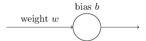
我们期望该神经元在输入 1 时输出 0。若神经元权重初始值为 0.6,偏移初始值为 0.9,则初始输出为 0.82,离预期输出还有一段距离。我们选择学习率 $\eta=0.15$,点击 Run 观察输出变化和二次代价函数的变化动画:
可以看到,神经元一直在“学习进步”,且“进步”神速,最终的输出也接近于 0。现在将权重初始值和偏移初始值都设为 2.0,再点击 Run 观察动画:
参数未变,结果造成学习速度减慢。仔细观察,开始的 150 个 epoch 权重和偏移几乎保持不变。过了这个点,神经元又变成了“进步”神速的好孩子。
我们经常把自学习与人类的学习作比较,这里神经元的学习过程显得反常。当人类发现自己错误的离谱时会学习较快,而大部分未优化的神经元却在错误中踌躇不前。
让我们来探究一下问题的缘由。神经元学习慢,等同于权重和偏移变化慢,等同于代价函数的偏导数 $\partial C/\partial w$ 和 $\partial C / \partial b$ 较小。我们的二次代价函数为
\begin{eqnarray} C = \frac{(y-a)^2}{2}, \label{54} \end{eqnarray}
其中,$a$ 是当训练输入 $x=1$ 时神经元的输出,$y=0$ 是期望输出。将 $a=\sigma(z), z = wx+b$ 代入上式,并求取偏导数可得
\begin{eqnarray} \frac{\partial C}{\partial w} & = & (a-y)\sigma'(z) x = a \sigma'(z) \label{55}\\ \frac{\partial C}{\partial b} & = & (a-y)\sigma'(z) = a \sigma'(z), \label{56} \end{eqnarray}
结合我们的 $\sigma$ 函数图像,即 sigmoid 函数图像:
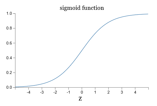
当神经元的输出接近于 0 时,曲线变得很平缓,所以 $\sigma'(z)$ 的值很小,结合公式 (\ref{55}) 和 (\ref{56}) 可知,$\partial C/\partial w$ 和 $\partial C / \partial b$ 的值很小。
介绍交叉熵代价函数
假设我们要训练如下的神经元,输入变量为 $x_1, x_2, ...$,对应的权重为 $w_1, w_2, ...$,偏移为 $b$:
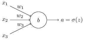
其中输出是 $a=\sigma(z), z = \sum_j w_j x_j+b$。对此,我们定义该神经元的交叉熵代价函数为
\begin{eqnarray} C = -\frac{1}{n} \sum_x \left[y \ln a + (1-y ) \ln (1-a) \right], \label{57} \end{eqnarray}
其中,$n$ 是所有训练数据的总和,$x$ 和 $y$ 是相应的输入和期望输出。为什么公式 (\ref{57}) 可以作为代价函数?
首先,由于 $a$ 的取值在 0, 1 之间,$y \ln a + (1-y) \ln (1-a)$ 为负,取反后公式 (\ref{57}) 非负。然后,当实际输出 $a$ 接近期望输出 $y$ 时,交叉熵接近于 0。这两点是代价函数的基本条件。将 $a = \sigma(z)$ 代入公式 (\ref{57}) 并计算交叉熵对权重的偏导,得
\begin{eqnarray} \frac{\partial C}{\partial w_j} & = & -\frac{1}{n} \sum_x \left( \frac{y }{\sigma(z)} -\frac{(1-y)}{1-\sigma(z)} \right) \frac{\partial \sigma}{\partial w_j} \label{58}\\ & = & -\frac{1}{n} \sum_x \left( \frac{y}{\sigma(z)} -\frac{(1-y)}{1-\sigma(z)} \right)\sigma'(z) x_j. \label{59} \end{eqnarray}
合并成一个分母,得
\begin{eqnarray} \frac{\partial C}{\partial w_j} & = & \frac{1}{n} \sum_x \frac{\sigma'(z) x_j}{\sigma(z) (1-\sigma(z))} (\sigma(z)-y). \label{60} \end{eqnarray}
由于 $\sigma'(z) = \sigma(z)(1-\sigma(z))$,上式还可以抵消,进一步简化为
\begin{eqnarray} \frac{\partial C}{\partial w_j} = \frac{1}{n} \sum_x x_j(\sigma(z)-y). \label{61} \end{eqnarray}
权重的学习速率由 $\sigma(z)-y$ 控制,误差越大,学习越快。二次代价函数 (\ref{55}) 中,正是由于 $\sigma'(z)$ 的存在,自学习的速率减慢,而公式 (\ref{61}) 消掉了这一项。同理,可得交叉熵对权重的偏导数为
\begin{eqnarray} \frac{\partial C}{\partial b} = \frac{1}{n} \sum_x (\sigma(z)-y). \label{62} \end{eqnarray}
同样,恼人的 $\sigma'(z)$ 也被消掉了。
让我们再来看一下之前动画,这次使用交叉熵作为代价函数,且学习率改为 $\eta=0.005$。第一个,权重初始值是 0.6,偏移初始值是 0.9,点击 Run。
意料之中,学习速度还是很快。第二个,权重和偏移初始值都为 2,点击 Run。
神经元还是学习迅速。你可能注意到了 $\eta$ 的变化,这会不会影响试验结果?其实,我们关心的不是神经元学习的绝对速度,而是学习速度本身的变化。
上述结论完全可以推广到多层多神经元的网络,定义交叉熵为
\begin{eqnarray} C = -\frac{1}{n} \sum_x \sum_j \left[y_j \ln a^L_j + (1-y_j) \ln (1-a^L_j) \right]. \label{63} \end{eqnarray}
那什么时候该用交叉熵而不是二次代价函数?对于 sigmoid 神经元,交叉熵几乎永远是更优选择,也被实践证明。
柔性最大值传输 softmax
通过将神经网络的输出由 sigmoid 换成 softmax 层可以进一步改善学习缓慢的问题。
对于输出层,其权重输入为 $z^L_j = \sum_{k} w^L_{jk} a^{L-1}_k + b^L_j$,施加 softmax 函数,输出层激励为
\begin{eqnarray} a^L_j = \frac{e^{z^L_j}}{\sum_k e^{z^L_k}}, \label{78} \end{eqnarray}
其中,分母是所有输出神经元输出之和。又是一个看起来意义不明的函数。如果我们将所有激励相加,会发现其值正好等于 1,
\begin{eqnarray} \sum_j a^L_j & = & \frac{\sum_j e^{z^L_j}}{\sum_k e^{z^L_k}} = 1. \label{79} \end{eqnarray}
当某一个激励增加时,其他的激励必须相应地减少以保证和不变。换句话说,如果将 softmax 作为输出层,神经网络的所有输出符合概率分布。这又是一个方便的特性,尤其对于手写数字识别来说,每个输出代表每个数字的概率,之前 sigmoid 的方案有可能会有如下的输出
[0.9, 0.3, 0.4, 0.1, 0.0, 0.4, 0.0, 0.0, 0.0, 0.1]
每个概率之间并没有联系,sigmoid 输出神经元只是各顾各的训练。而且人们拿到这个结果肯定会非常疑惑,为啥概率相加不等于 1?
过拟合和正则化
诺贝尔物理学奖获得者费米曾经和他的同事讨论一个数学模型。该模型能够很好地解释实验结果,但费米仍有疑虑。他问该模型用了多少个自由变量,同事回答四个。费米回答:“我记得我朋友冯诺依曼曾经说过,四个变量我能描述一头大象,五个变量就能让他转鼻子了”。
拥有大量自由变量的模型很容易就描述大部分实验现象。但是不能说符合实验现象的模型就是好模型。有足够自由变量的模型中,几乎可以描述任何给定大小的数据集,但没有抓住现象背后的本质。这种情况下,模型只能适用于现有数据,面对新的情况却束手无策。模型的真正考验,是它有能力对未出现的现象做出预言。
费米和诺依曼对四变量的模型就产生了质疑。而我们手写数字识别系统有 30 个隐藏神经元,有将近 24000 个变量!若是 100 个隐藏神经元,那就有近 80000 个变量!这么多变量,不禁要问,结果可信么?会出现费米和诺依曼担心的问题么?
让我们来模拟一下这种情况的发生。我们使用 30 个隐藏神经元,但我们不使用 50000 个 MNIST 训练图像,相反,只是用 1000 个训练图像。这样,问题会更显著。训练使用交叉熵函数,学习率 $\eta=0.5$,mini-batch 大小为 10,训练 400 个epochs。让我们用 network2 来观察变化。
import mnist_loader
training_data, validation_data, test_data = mnist_loader.load_data_wrapper()
import network2
net = network2.Network([784, 30, 10], cost=network2.CrossEntropyCost)
net.large_weight_initializer()
net.SGD(training_data[:1000], 400, 10, 0.5, evaluation_data=test_data, monitor_evaluation_accuracy=True, monitor_training_cost=True)
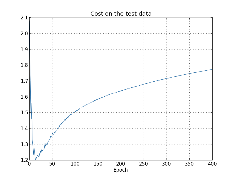
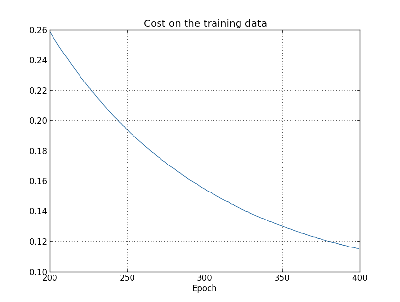
首先是代价函数随学习进度的变化图像:
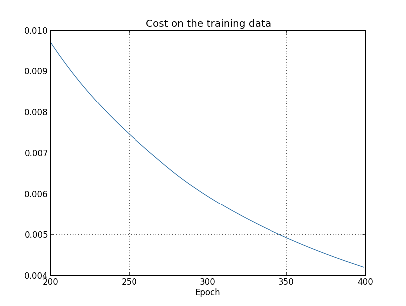
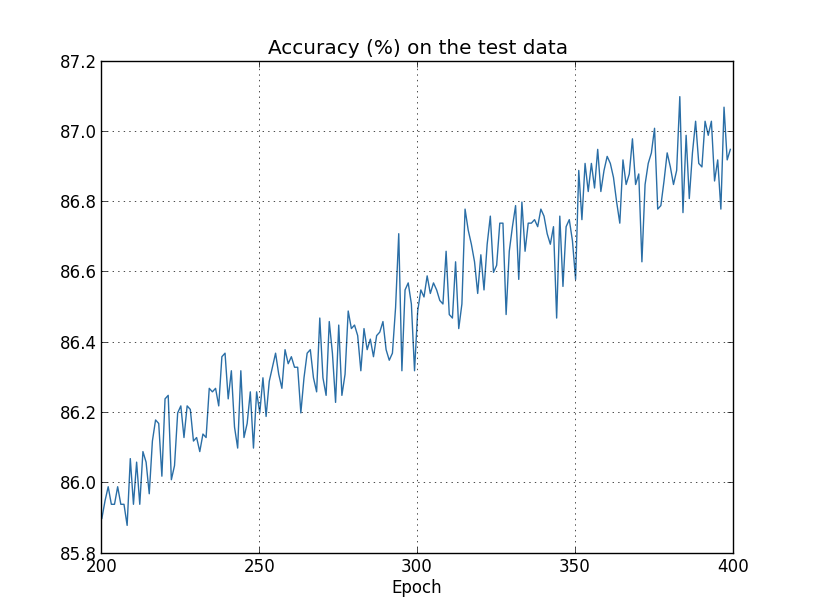
看起来不错,代价不断减小,似乎说明我们的神经网络一直在进步。但是测试集上识别率却不是那么回事:
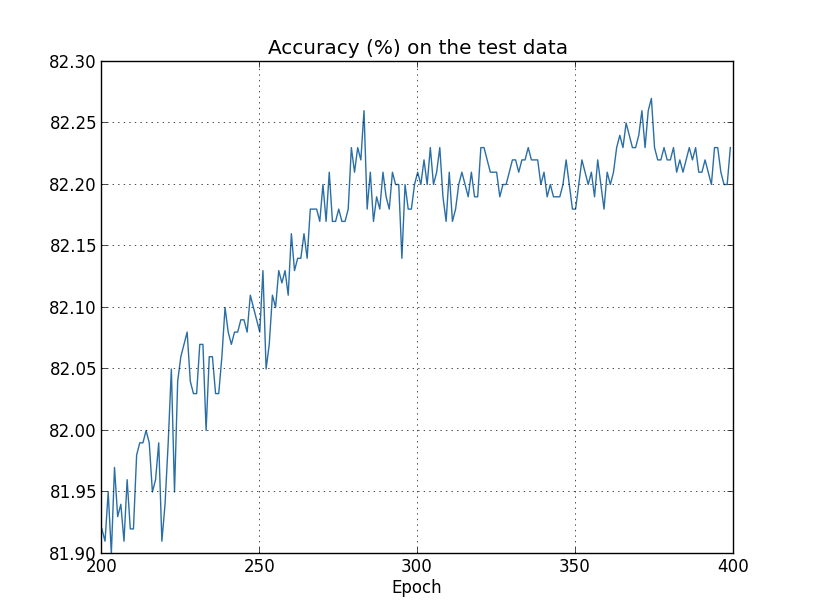
280 个 epoch 之后,识别率处于波动稳定状态,且远低于之前达到的 95% 识别率。训练数据的交叉熵和测试集的实际结果截然不同,出现了费米担心的问题。可以说,280 个 epoch 之后的学习完全无用,标准说法是过拟合 overfitting。
让我们在做一点更直观的比较:训练集和测试集的交叉熵横向对比,及识别率横向对比。
交叉熵仅仅下降了 15 个 epoch,之后就一路飙高,持续恶化。这是我们模型过拟合的又一个标志。这里有个小疑问,epoch 15 和 epoch 280 哪个属于开始过拟合?从实践的角度看,我们真正的关心的是测试集(更接近真实情况)上的识别率,交叉熵只是算法的附带物,所以我们认为,epoch 280 之后,过拟合开始占据神经网络的学习过程。
下面是训练集的识别率变化:
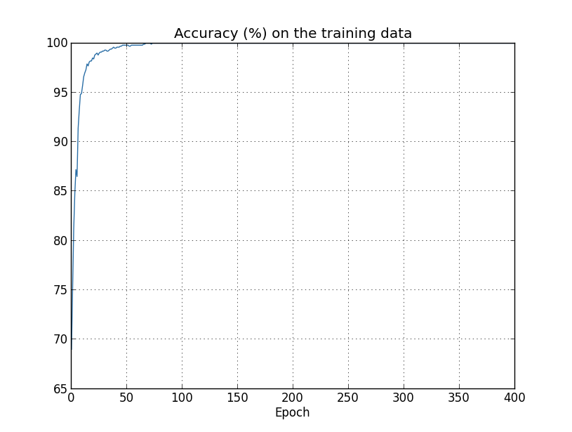
我们的模型能够 100% 地描述 1000 个训练图像,实际却不能很好地分类测试数字。
最明显的检测过拟合的方法是观察测试集上识别率的变化。如果发现测试集识别率不再改善,就应该停止训练。这也是之前文章-代码实现为什么要再引入验证集的原因,毕竟测试集是最终判定结果用的,应该与训练过程彻底分离。
training_data, validation_data, test_data = mnist_loader.load_data_wrapper()
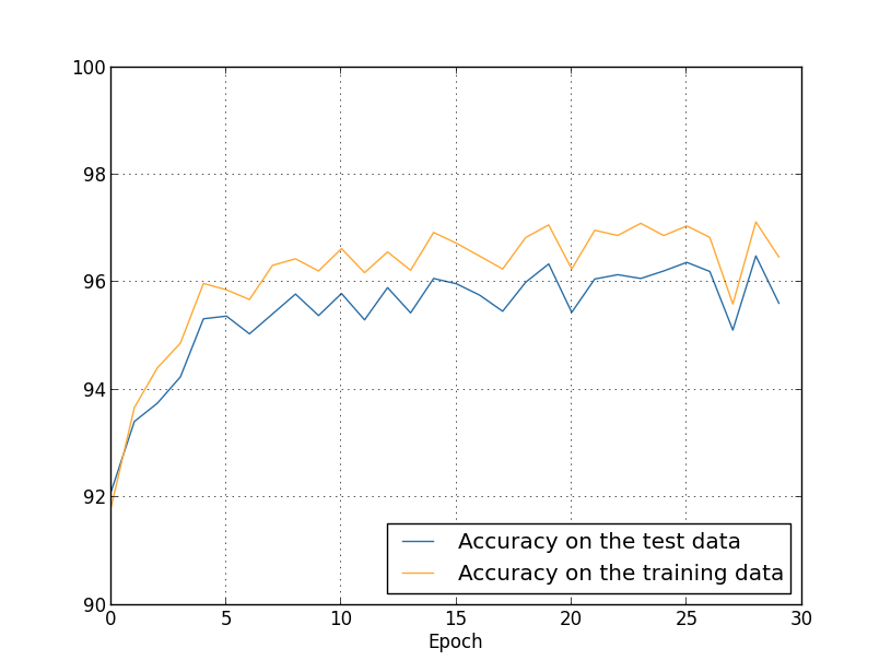
我们一直在讨论 1000 个训练图片的过拟合问题,那 50000 个图片结果还是一样吗?这里给出结果:
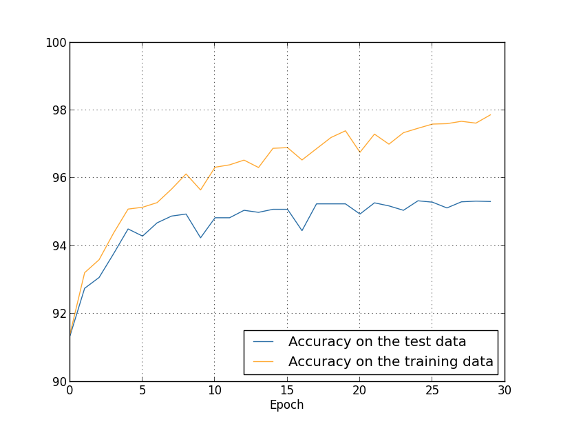
可以看到,过拟合不再那么明显了,训练集的识别率只比测试集高 1.5% 左右。这也间接说明,大量训练数据下神经网络难以达到过拟合。不过训练集并不是那么容易获得的。
正则化 Regularization
首先要明确一点,我们并不想减少网络中变量的数目,我们需要这种特性来描述现实世界复杂的变化。
正则化方法能够缓解过拟合问题,最常用的是权重衰减法或者叫 $L_2$ 正则化。$L_2$ 正则化只是在原先的代价函数中加入一个正则项:
\begin{eqnarray} C = -\frac{1}{n} \sum_{xj} \left[ y_j \ln a^L_j+(1-y_j) \ln (1-a^L_j)\right] + \frac{\lambda}{2n} \sum_w w^2. \label{85} \end{eqnarray}
等式右边第一项是交叉熵,第二项是网络中所有权重的平方和,并乘以系数 $\lambda /2n$,其中 $\lambda > 0$,称作正则化参数。
正则化不只适用于交叉熵代价函数,二次代价函数也可以使用:
\begin{eqnarray} C = \frac{1}{2n} \sum_x |y-a^L|^2 + \frac{\lambda}{2n} \sum_w w^2. \label{86} \end{eqnarray}
总结下来就是
\begin{eqnarray}
C = C_0 + \frac{\lambda}{2n}
\sum_w w^2,
\label{87}
\end{eqnarray}
其中 $C_0$ 是未正则化的代价函数。观察该式,可以发现正则化逼迫自学习过程选择更小的权重,权重越大,代价也越高。由于代价函数的变换,随机梯度下降法中偏导数的计算也要随之改变:
\begin{eqnarray} \frac{\partial C}{\partial w} & = & \frac{\partial C_0}{\partial w} + \frac{\lambda}{n} w \label{88}\\ \frac{\partial C}{\partial b} & = & \frac{\partial C_0}{\partial b}. \label{89} \end{eqnarray}
$\partial C_0 / \partial w$ 和 $\partial C_0 / \partial b$ 仍让可以用上一篇的反向传播算法求得。对偏移的偏导数并没有改变,所以据梯度下降法学习规则仍为:
\begin{eqnarray} b & \rightarrow & b -\eta \frac{\partial C_0}{\partial b}. \label{90} \end{eqnarray}
而权重的自学习规则则变成:
\begin{eqnarray} w & \rightarrow & w-\eta \frac{\partial C_0}{\partial w}-\frac{\eta \lambda}{n} w \label{91}\\ & = & \left(1-\frac{\eta \lambda}{n}\right) w -\eta \frac{\partial C_0}{\partial w}. \label{92} \end{eqnarray}
可以看到,权重 $w$ 乘以了一个小于 1 的系数 $1-\frac{\eta \lambda}{n}$,称为权重衰减,有减小权重的趋势。而后一项由于偏导有正有负,所以权重值并不是单调递减,两项相加,彼此制约。
以上是梯度下降法,随机梯度下降法也只要做相应的调整:
\begin{eqnarray} w \rightarrow \left(1-\frac{\eta \lambda}{n}\right) w -\frac{\eta}{m} \sum_x \frac{\partial C_x}{\partial w}, \label{93} \end{eqnarray}
\begin{eqnarray} b \rightarrow b - \frac{\eta}{m} \sum_x \frac{\partial C_x}{\partial b}, \label{94} \end{eqnarray}
其中,求和是对一个 mini-batch 内所有数据的求和。
让我们实验一下。这次在 network2 中加入正则化参数 $\lambda=0.1$。对比之前 1000 个训练数据集的结果:
import mnist_loader
training_data, validation_data, test_data = mnist_loader.load_data_wrapper()
import network2
net = network2.Network([784, 30, 10], cost=network2.CrossEntropyCost)
net.large_weight_initializer()
net.SGD(training_data[:1000], 400, 10, 0.5,
        evaluation_data=test_data, lmbda = 0.1,
        monitor_evaluation_cost=True, monitor_evaluation_accuracy=True,
        monitor_training_cost=True, monitor_training_accuracy=True)
训练集的交叉熵代价看来没什么问题:
但这次识别率却是一直在上升:
我们在试一下 50000 个训练数据的情况:
训练集和测试集的识别率只差 1% 左右,而正则化之前这一值是 1.5%。
用以下参数
net = network2.Network([784, 100, 10], cost=network2.CrossEntropyCost)
net.large_weight_initializer()
net.SGD(training_data, 60, 10, 0.1, lmbda=5.0,
      evaluation_data=validation_data,
      monitor_evaluation_accuracy=True)
识别率提高到 98%。你可以认为,由于过拟合的存在,神经网络模型易陷入局部最优解,正则之后,跳出局部最优,滚向全局最优,最终带来识别率的提升。
为什么正则化能抑制过拟合
从正则化的结果来看,似乎权重值越小越能抑制过拟合。
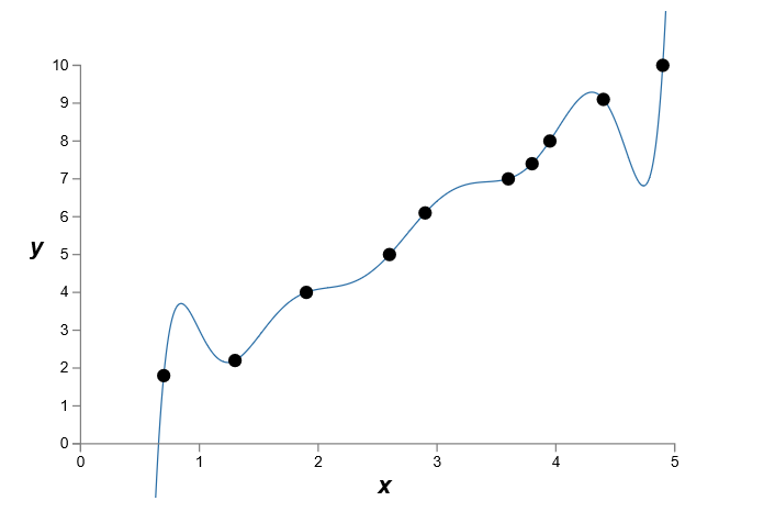
让我们看一个经典的例子,假设要对下图所示的点建立一个模型:
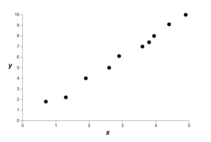
数一下,有 10 个点,那可以用一个 9 次函数精确地描述它,$y = a_0 x^9 + a_1 x^8 + \ldots + a_9$:
如果允许一些误差,也可以使用一个简单的线性模型:
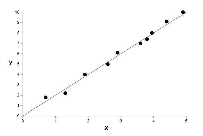
那么,哪个才是更好的模型?哪个才能描述还未出现的新点?实践表明,允许一定误差的模型更符合实际情况。现实世界伴随着大量不确定性,传感器采集的噪声和仪器本身的精度都会给训练集加入一定的噪声,这样,后一个模型便在预测新点时占据了优势。
回到我们的神经网络,当输入因为某些噪声剧烈变化时,较小的权值 $w$ 能够防止网络整体特性改变过大,网络也就不会去“学习”那些没用的噪声信息了。相反,对于手写数字图像那些重复的特征,神经网络在一遍遍的 mini-batch 中,“铭记在心”。
人们也称这个思想为奥卡姆剃刀原理:当两个假说具有完全相同的解释力和预测力时,我们以那个较为简单的假说作为讨论依据。
其他抑制过拟合的方法
当然还有很多抑制过拟合的方法,比如:
$L_1$ 正则化,即换一个正则函数。
dropout:学习过程中随机删去一些神经元。
人工扩展训练集:这也是我比较喜欢的一个方法,可以通过平移、缩放、旋转、elastic distortions 等扩展数据集。扩展数据简单粗暴有效,微软研究院的研究员用 elastic distortions 扩展数据后,就将 MNIST 识别率提高到了 99.3%。
改进权重初始化
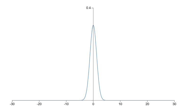
我们在初始化权重和偏移时,选择高斯随机,均值为 0,标准差为 1。权重输入为 $z = \sum_j w_j x_j+b$,随着输入神经元数目的增加,标准差也随之增加,例如 1000 个神经元,其正太分布曲线为
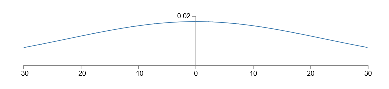
曲线非常平坦,意味着 $z \gg 1, z \ll -1$ 的可能性都大大增加,输出 $\sigma(z)$ 极有可能饱和,出现过拟合的现象。解决的方法也非常简单,初始化时标准差选为 $1/\sqrt{n_{\rm in}}$。
代码
以下是 network2.py 的源码(当然我不是写的啦,Michael Nielsen 的杰作),所用技术和算法已在上文逐一阐述。
"""network2.py
~~~~~~~~~~~~~~

An improved version of network.py, implementing the stochastic
gradient descent learning algorithm for a feedforward neural network.
Improvements include the addition of the cross-entropy cost function,
regularization, and better initialization of network weights.  Note
that I have focused on making the code simple, easily readable, and
easily modifiable.  It is not optimized, and omits many desirable
features.

"""

#### Libraries
# Standard library
import json
import random
import sys

# Third-party libraries
import numpy as np


#### Define the quadratic and cross-entropy cost functions

class QuadraticCost(object):

    @staticmethod
    def fn(a, y):
        """Return the cost associated with an output ``a`` and desired output
        ``y``.

        """
        return 0.5*np.linalg.norm(a-y)**2

    @staticmethod
    def delta(z, a, y):
        """Return the error delta from the output layer."""
        return (a-y) * sigmoid_prime(z)


class CrossEntropyCost(object):

    @staticmethod
    def fn(a, y):
        """Return the cost associated with an output ``a`` and desired output
        ``y``.  Note that np.nan_to_num is used to ensure numerical
        stability.  In particular, if both ``a`` and ``y`` have a 1.0
        in the same slot, then the expression (1-y)*np.log(1-a)
        returns nan.  The np.nan_to_num ensures that that is converted
        to the correct value (0.0).

        """
        return np.sum(np.nan_to_num(-y*np.log(a)-(1-y)*np.log(1-a)))

    @staticmethod
    def delta(z, a, y):
        """Return the error delta from the output layer.  Note that the
        parameter ``z`` is not used by the method.  It is included in
        the method's parameters in order to make the interface
        consistent with the delta method for other cost classes.

        """
        return (a-y)


#### Main Network class
class Network(object):

    def __init__(self, sizes, cost=CrossEntropyCost):
        """The list ``sizes`` contains the number of neurons in the respective
        layers of the network.  For example, if the list was [2, 3, 1]
        then it would be a three-layer network, with the first layer
        containing 2 neurons, the second layer 3 neurons, and the
        third layer 1 neuron.  The biases and weights for the network
        are initialized randomly, using
        ``self.default_weight_initializer`` (see docstring for that
        method).

        """
        self.num_layers = len(sizes)
        self.sizes = sizes
        self.default_weight_initializer()
        self.cost=cost

    def default_weight_initializer(self):
        """Initialize each weight using a Gaussian distribution with mean 0
        and standard deviation 1 over the square root of the number of
        weights connecting to the same neuron.  Initialize the biases
        using a Gaussian distribution with mean 0 and standard
        deviation 1.

        Note that the first layer is assumed to be an input layer, and
        by convention we won't set any biases for those neurons, since
        biases are only ever used in computing the outputs from later
        layers.

        """
        self.biases = [np.random.randn(y, 1) for y in self.sizes[1:]]
        self.weights = [np.random.randn(y, x)/np.sqrt(x)
                        for x, y in zip(self.sizes[:-1], self.sizes[1:])]

    def large_weight_initializer(self):
        """Initialize the weights using a Gaussian distribution with mean 0
        and standard deviation 1.  Initialize the biases using a
        Gaussian distribution with mean 0 and standard deviation 1.

        Note that the first layer is assumed to be an input layer, and
        by convention we won't set any biases for those neurons, since
        biases are only ever used in computing the outputs from later
        layers.

        This weight and bias initializer uses the same approach as in
        Chapter 1, and is included for purposes of comparison.  It
        will usually be better to use the default weight initializer
        instead.

        """
        self.biases = [np.random.randn(y, 1) for y in self.sizes[1:]]
        self.weights = [np.random.randn(y, x)
                        for x, y in zip(self.sizes[:-1], self.sizes[1:])]

    def feedforward(self, a):
        """Return the output of the network if ``a`` is input."""
        for b, w in zip(self.biases, self.weights):
            a = sigmoid(np.dot(w, a)+b)
        return a

    def SGD(self, training_data, epochs, mini_batch_size, eta,
            lmbda = 0.0,
            evaluation_data=None,
            monitor_evaluation_cost=False,
            monitor_evaluation_accuracy=False,
            monitor_training_cost=False,
            monitor_training_accuracy=False):
        """Train the neural network using mini-batch stochastic gradient
        descent.  The ``training_data`` is a list of tuples ``(x, y)``
        representing the training inputs and the desired outputs.  The
        other non-optional parameters are self-explanatory, as is the
        regularization parameter ``lmbda``.  The method also accepts
        ``evaluation_data``, usually either the validation or test
        data.  We can monitor the cost and accuracy on either the
        evaluation data or the training data, by setting the
        appropriate flags.  The method returns a tuple containing four
        lists: the (per-epoch) costs on the evaluation data, the
        accuracies on the evaluation data, the costs on the training
        data, and the accuracies on the training data.  All values are
        evaluated at the end of each training epoch.  So, for example,
        if we train for 30 epochs, then the first element of the tuple
        will be a 30-element list containing the cost on the
        evaluation data at the end of each epoch. Note that the lists
        are empty if the corresponding flag is not set.

        """
        if evaluation_data: n_data = len(evaluation_data)
        n = len(training_data)
        evaluation_cost, evaluation_accuracy = [], []
        training_cost, training_accuracy = [], []
        for j in xrange(epochs):
            random.shuffle(training_data)
            mini_batches = [
                training_data[k:k+mini_batch_size]
                for k in xrange(0, n, mini_batch_size)]
            for mini_batch in mini_batches:
                self.update_mini_batch(
                    mini_batch, eta, lmbda, len(training_data))
            print "Epoch %s training complete" % j
            if monitor_training_cost:
                cost = self.total_cost(training_data, lmbda)
                training_cost.append(cost)
                print "Cost on training data: {}".format(cost)
            if monitor_training_accuracy:
                accuracy = self.accuracy(training_data, convert=True)
                training_accuracy.append(accuracy)
                print "Accuracy on training data: {} / {}".format(
                    accuracy, n)
            if monitor_evaluation_cost:
                cost = self.total_cost(evaluation_data, lmbda, convert=True)
                evaluation_cost.append(cost)
                print "Cost on evaluation data: {}".format(cost)
            if monitor_evaluation_accuracy:
                accuracy = self.accuracy(evaluation_data)
                evaluation_accuracy.append(accuracy)
                print "Accuracy on evaluation data: {} / {}".format(
                    self.accuracy(evaluation_data), n_data)
            print
        return evaluation_cost, evaluation_accuracy, \
            training_cost, training_accuracy

    def update_mini_batch(self, mini_batch, eta, lmbda, n):
        """Update the network's weights and biases by applying gradient
        descent using backpropagation to a single mini batch.  The
        ``mini_batch`` is a list of tuples ``(x, y)``, ``eta`` is the
        learning rate, ``lmbda`` is the regularization parameter, and
        ``n`` is the total size of the training data set.

        """
        nabla_b = [np.zeros(b.shape) for b in self.biases]
        nabla_w = [np.zeros(w.shape) for w in self.weights]
        for x, y in mini_batch:
            delta_nabla_b, delta_nabla_w = self.backprop(x, y)
            nabla_b = [nb+dnb for nb, dnb in zip(nabla_b, delta_nabla_b)]
            nabla_w = [nw+dnw for nw, dnw in zip(nabla_w, delta_nabla_w)]
        self.weights = [(1-eta*(lmbda/n))*w-(eta/len(mini_batch))*nw
                        for w, nw in zip(self.weights, nabla_w)]
        self.biases = [b-(eta/len(mini_batch))*nb
                       for b, nb in zip(self.biases, nabla_b)]

    def backprop(self, x, y):
        """Return a tuple ``(nabla_b, nabla_w)`` representing the
        gradient for the cost function C_x.  ``nabla_b`` and
        ``nabla_w`` are layer-by-layer lists of numpy arrays, similar
        to ``self.biases`` and ``self.weights``."""
        nabla_b = [np.zeros(b.shape) for b in self.biases]
        nabla_w = [np.zeros(w.shape) for w in self.weights]
        # feedforward
        activation = x
        activations = [x] # list to store all the activations, layer by layer
        zs = [] # list to store all the z vectors, layer by layer
        for b, w in zip(self.biases, self.weights):
            z = np.dot(w, activation)+b
            zs.append(z)
            activation = sigmoid(z)
            activations.append(activation)
        # backward pass
        delta = (self.cost).delta(zs[-1], activations[-1], y)
        nabla_b[-1] = delta
        nabla_w[-1] = np.dot(delta, activations[-2].transpose())
        # Note that the variable l in the loop below is used a little
        # differently to the notation in Chapter 2 of the book.  Here,
        # l = 1 means the last layer of neurons, l = 2 is the
        # second-last layer, and so on.  It's a renumbering of the
        # scheme in the book, used here to take advantage of the fact
        # that Python can use negative indices in lists.
        for l in xrange(2, self.num_layers):
            z = zs[-l]
            sp = sigmoid_prime(z)
            delta = np.dot(self.weights[-l+1].transpose(), delta) * sp
            nabla_b[-l] = delta
            nabla_w[-l] = np.dot(delta, activations[-l-1].transpose())
        return (nabla_b, nabla_w)

    def accuracy(self, data, convert=False):
        """Return the number of inputs in ``data`` for which the neural
        network outputs the correct result. The neural network's
        output is assumed to be the index of whichever neuron in the
        final layer has the highest activation.

        The flag ``convert`` should be set to False if the data set is
        validation or test data (the usual case), and to True if the
        data set is the training data. The need for this flag arises
        due to differences in the way the results ``y`` are
        represented in the different data sets.  In particular, it
        flags whether we need to convert between the different
        representations.  It may seem strange to use different
        representations for the different data sets.  Why not use the
        same representation for all three data sets?  It's done for
        efficiency reasons -- the program usually evaluates the cost
        on the training data and the accuracy on other data sets.
        These are different types of computations, and using different
        representations speeds things up.  More details on the
        representations can be found in
        mnist_loader.load_data_wrapper.

        """
        if convert:
            results = [(np.argmax(self.feedforward(x)), np.argmax(y))
                       for (x, y) in data]
        else:
            results = [(np.argmax(self.feedforward(x)), y)
                        for (x, y) in data]
        return sum(int(x == y) for (x, y) in results)

    def total_cost(self, data, lmbda, convert=False):
        """Return the total cost for the data set ``data``.  The flag
        ``convert`` should be set to False if the data set is the
        training data (the usual case), and to True if the data set is
        the validation or test data.  See comments on the similar (but
        reversed) convention for the ``accuracy`` method, above.
        """
        cost = 0.0
        for x, y in data:
            a = self.feedforward(x)
            if convert: y = vectorized_result(y)
            cost += self.cost.fn(a, y)/len(data)
        cost += 0.5*(lmbda/len(data))*sum(
            np.linalg.norm(w)**2 for w in self.weights)
        return cost

    def save(self, filename):
        """Save the neural network to the file ``filename``."""
        data = {"sizes": self.sizes,
                "weights": [w.tolist() for w in self.weights],
                "biases": [b.tolist() for b in self.biases],
                "cost": str(self.cost.__name__)}
        f = open(filename, "w")
        json.dump(data, f)
        f.close()

#### Loading a Network
def load(filename):
    """Load a neural network from the file ``filename``.  Returns an
    instance of Network.

    """
    f = open(filename, "r")
    data = json.load(f)
    f.close()
    cost = getattr(sys.modules[__name__], data["cost"])
    net = Network(data["sizes"], cost=cost)
    net.weights = [np.array(w) for w in data["weights"]]
    net.biases = [np.array(b) for b in data["biases"]]
    return net

#### Miscellaneous functions
def vectorized_result(j):
    """Return a 10-dimensional unit vector with a 1.0 in the j'th position
    and zeroes elsewhere.  This is used to convert a digit (0...9)
    into a corresponding desired output from the neural network.

    """
    e = np.zeros((10, 1))
    e[j] = 1.0
    return e

def sigmoid(z):
    """The sigmoid function."""
    return 1.0/(1.0+np.exp(-z))

def sigmoid_prime(z):
    """Derivative of the sigmoid function."""
    return sigmoid(z)*(1-sigmoid(z))