基于 BP 神经网络的手写体数字识别 - 设计与实现
(基于 BP 神经网络的识别手写体数字, Part 2)
手写体数字识别的神经网络结构
上一篇文章中我们简单介绍了神经网络,接下来让我们运用到主题中 —— 手写体数字识别。
手写数字识别可以分为两大子问题。第一是如何将一串数字分割成单个的数字,第二是识别单个数字。我们将专注于解决第二个问题,因为分割问题并不难,而且和我们的主题——神经网络相差甚远。
为了识别单个的数字,我们将使用三层神经网络:

输入层的神经元将对输入的像素值编码。神经网络的训练数据包含了 $28 \times 28$ 像素的扫描图,所以输入层有 $784 = 28 \times 28$ 个神经元。为了简便起见,上图中没有 $784$ 个输入神经元全部画出。每一个像素是灰度值,$0.0$ 代表白色,$1.0$ 代表黑色,两者之间的为逐渐变黑的灰色。
第二层是隐藏层。让我们记隐藏层的神经元数量为 $n$,我们将对 $n$ 的不同值实验。上图中,$n=15$。
输出层包含 $10$ 个神经元。如果第一个输出被激活了,即 $\mbox{output} \approx 1$,意味着神经网络判定当前数字为 $0$。如果第二个输出神经元被激活,则神经网络认为当前数字很有可能为 $1$。以此类推。最后对 $10$ 个输出神经元进行排序,哪个最高说明神经网络认为其最有可能。比如第 $6$ 个神经元输出最高,则输入图像最有可能是数字 $6$。
你可能会想为什么会用十个输出神经元?毕竟我们的目标是判断出每一个图片对应的数字,理论上,四个输出的组合就可以编码,$2^4 = 16$ 完全可以包含 $10$ 个值。要回答这个问题还是得靠实验:我们对两种输出编码方案都做了实验,用 $10$ 个输出的效果更好。让我们做一个启发式的思考,用四个 bit 来唯一确定一个数字,意味着得百分百识别出图像,说一不二。而有些时候字确实写的难以辨认,连人类自己都只能说‘大概是 4 或者 9’这种话,这时候,给出 $10$ 个数字的概率更符合人脑的思维方式。
基于梯度下降法学习
现在我们已经设计出神经网络的结构了,那如何识别出数字呢?第一件事是找到训练集。我们将使用 MNIST 数据集。MNIST 是经过修改的 NIST 数据子集,NIST 即 United States' National Institute of Standards and Technology。以下是部分数据:
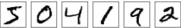
图像已经被分割成单个的数字,而且没有噪点等,不需要做图像预处理。MNIST 数据集包括两部分,第一部分包含 60000 个图像,被用作训练数据。这些图像来自 250 个人,半数来自美国人口普查局的员工,另外半数是高中生。图片是 $28 \times 28$ 的灰度图。第二部分是 10000 张图片的测试集。我们将使用测试集来评估人工神经网络的学习效果。为了取得更好的测试效果,测试集来自另外 250 个人。这样,测试集和训练集的完全不同能够更好验证结果。
我们将使用 $x$ 来标记训练输入。虽然图片是一个二维数组,不过我们输入会采用 $28 \times 28 = 784$ 的向量。向量中的每一项为图片每一个像素的灰度值。输出我们将记为输出向量 $y = y(x)$。如果一个训练图片是数字 6,则 $y(x) = (0, 0, 0, 0, 0, 0, 1, 0, 0, 0)^\mathrm{T}$。请注意,$\mathrm{T}$ 是转置操作。
算法的目标是找到权重和偏移,对于所有训练输入 $x$,网络都能够输出正确的 $y(x)$。为了量化我们与目标的接近程度,定义以下的代价函数:
\begin{eqnarray} C(w,b) \equiv \frac{1}{2n} \sum_x | y(x) - a|^2. \label{6} \end{eqnarray}
这里,记 $w$ 为网络所有的权重集,$b$ 为所有的偏移,$n$ 为训练输入的总数,$a$ 为实际的输出向量,求和是对所有训练输入而言。当然,$a$ 应该是 $x,w,b$ 的函数。记号 $| v |$ 为向量 $v$ 的长度。我们称 $C$ 为二次代价函数,其实就是均方差啦, MSE (mean squared error)。可以看出,该代价函数为非负值,并且,当所有训练数据的 $y(x)$ 接近实际输出 $a$ 时,代价函数 $C(w,b) \approx 0$。所以,当神经网络工作良好的时候,$C(w,b)$ 很小,相反,该值会很大,即训练集中有很大一部分预期输出 $y(x)$ 和实际输出 $a$ 不符。我们训练算法的目标,就是找到一组权重和偏移,让误差尽可能的小。
为什么会用二次函数误差?毕竟我们感兴趣的是能被正确分类的图片数量。为什么不直接以图片数量为目标,比如目标是识别的数量最大化?问题是,正确分类图像的数量不是权值和偏置的光滑函数,大部分情况下,变量的变化不会导致识别数量的变化,也就难以调整权重和偏移。
你可能还会好奇,二次函数是最好的选择吗?其他的代价函数会不会得到完全不同的权值和偏移,效果更好呢?事实上,确实有更好的代价函数,以后的文章还会继续探讨。不过,本文继续使用二次函数,它对我们理解神经网络的基本自学习过程非常有益。
接下来,我们介绍梯度下降法,它可以用来解决最小化问题。
假设我们要最小化函数 $C(v), v=v_1,v_2$。该函数图像为:
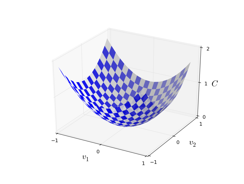
我们要找到 $C$ 的全局最小值。一种做法是计算函数的导数,找到各个极值。课本上的导数很好求解。不幸的是,现实生活中,问题所代表的函数经常包含过多的变量。尤其是神经网络中,有数以万计的权值和偏移,不可能直接求取极值。
幸好还有其他方法。让我们换种思维方式,对比那个函数图像,将函数看作一个山谷,并假设有一个小球沿着山谷斜坡滑动。直觉告诉我们小球最终会滑向坡底。也许这就能用来找到最小值?我们为“小球”随机选择一个起点,然后模拟“小球”沿斜坡滑动。“小球”运动的方向可以通过偏导数确定,这些偏导数包含了山谷形状的信息。
是否需要牛顿力学公式来获取小球的运动,考虑摩擦力和重力呢?并不需要,我们是在制定一个最小化 $C$ 的算法,而不是去精确模拟物理学规律。
让我们记球在 $v_1$ 方向移动了很小的量 $\Delta v_1$,在 $v_2$ 的方向移动了 $\Delta v_2$,总的 $C$ 的改变量为:
\begin{eqnarray} \Delta C \approx \frac{\partial C}{\partial v_1} \Delta v_1 + \frac{\partial C}{\partial v_2} \Delta v_2. \label{7} \end{eqnarray}
我们目标是找到一组 $\Delta v_1$ 和 $\Delta v_2$,使 $\Delta C$ 为负,即使球向谷底滚去。接下来记 $\Delta v \equiv (\Delta v_1, \Delta v_2)^T$ 为 $v$ 的总变化,并且记梯度向量 $\nabla C$ 为:
\begin{eqnarray} \nabla C \equiv \left( \frac{\partial C}{\partial v_1}, \frac{\partial C}{\partial v_2} \right)^T. \label{8} \end{eqnarray}
其中梯度向量符号 $\nabla C$ 会比较抽象,因为它纯粹就是一个数学上的概念。有了梯度符号,我们可以将式 (\ref{8}) 改写为
\begin{eqnarray} \Delta C \approx \nabla C \cdot \Delta v. \label{9} \end{eqnarray}
从该式可以看出,梯度向量 $\nabla C$ 将 $v$ 的变化反应到 $C$ 中,且我们也找到了如何让 $\Delta C$ 为负的方法。尤其是当我们选择
\begin{eqnarray} \Delta v = -\eta \nabla C, \label{10} \end{eqnarray}
当 $\eta$ 是一个很小的正参数时(其实该参数就是学习率),公式 (\ref{9}) 表明 $\Delta C \approx -\eta\nabla C \cdot \nabla C = -\eta |\nabla C|^2$。因为 $| \nabla C|^2 \geq 0$,能保证 $\Delta C \leq 0$。这正是我们需要的特性!在梯度下降学习法中,我们使用公式 (\ref{10}) 计算 $\Delta v$,然后移动球到新的位置:
\begin{eqnarray} v \rightarrow v' = v -\eta \nabla C. \label{11} \end{eqnarray}
然后不停使用这一公式计算下一步,直到 $C$ 不再减小为止,即找到了全局最小值。
总结一下,首先重复计算梯度 $\nabla C$,然后向相反方向移动,画成图就是
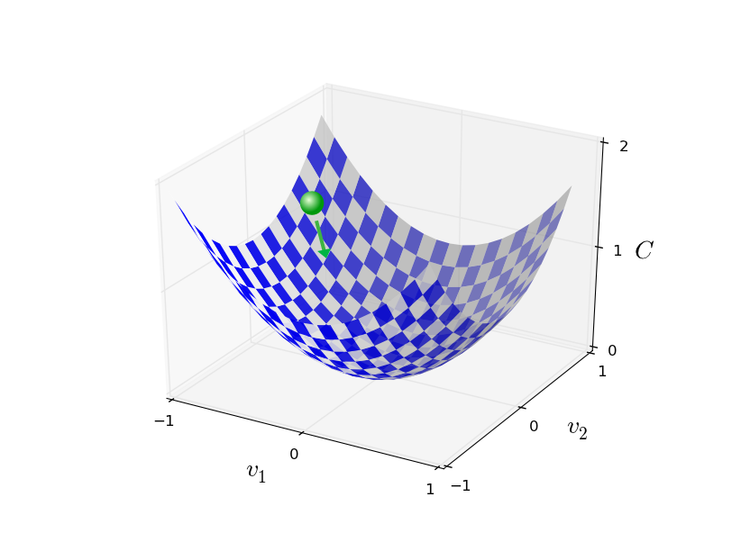
请注意,上述梯度下降的规则并没有复制出真正的物理运动。在真实生活中,球有动量,滚向谷底后还会继续滚上去,在摩擦力的作用下才会最终停下。但我们的算法中没这么复杂。
为了使算法正常工作,公式 (\ref{9}) 中的学习率 $\eta$ 要尽可能的小,不然最终可能 $\Delta C > 0$。同时学习率不能过小,不然会导致每一次迭代中 $\Delta v$ 过小,算法工作会非常慢。
尽管到现在我们一直用两个变量的函数 $C$ 举例。但其实对于多变量的函数,这仍是适用的。假设 $C$ 有 $m$ 个变量,$v_1,..., v_m$,那么变化 $\Delta C$ 为
\begin{eqnarray} \Delta C \approx \nabla C \cdot \Delta v, \label{12} \end{eqnarray}
其中 $\Delta v = (\Delta v_1,\ldots, \Delta v_m)^T$,梯度向量 $\nabla C$ 为
\begin{eqnarray} \nabla C \equiv \left(\frac{\partial C}{\partial v_1}, \ldots, \frac{\partial C}{\partial v_m}\right)^T. \label{13} \end{eqnarray}
梯度下降法虽然简单,但实际上很有效,也是一个经典的最优化方法,在神经网络中我们将用它来寻找代价函数的最小值。
同时,人们研究了大量梯度下降法的变种,包括去模拟真实的物理学,但都效果不好。因为这些变种算法不光计算一次偏导数,还需要计算二次偏导,这对计算机来说是巨大的挑战,尤其是有着上百万神经元的神经网络。
我们将使用梯度下降法来来找到权重 $w_k$ 和偏移 $b_l$。类比上述的梯度法,这里变量 $v_j$ 即为权重和偏移,而梯度 $\nabla C$ 为 $\partial C / \partial w_k$ 和 $\partial C/ \partial b_l$。梯度下降的更新规则如下:
\begin{eqnarray} w_k & \rightarrow & w_k' = w_k-\eta \frac{\partial C}{\partial w_k} \label{16}\\ b_l & \rightarrow & b_l' = b_l-\eta \frac{\partial C}{\partial b_l}. \label{17} \end{eqnarray}
重复上述规则,找到代价函数的最小值,实现神经网络的自学习。
在适用梯度下降法时仍有一些挑战,比如公式 (\ref{6}) 中代价函数是每一个训练样本的误差 $C_x \equiv \frac{|y(x)-a|^2}{2}$ 的平均值。这意味着计算梯度时,需要每一个训练样本计算梯度。当样本数量很多时,就会造成性能的问题。
随机梯度下降法能够解决这一问题,加速学习过程。算法每次随机从训练输入中选取 $m$ 个数据,$X_1, X_2,\ldots, X_m $,记为 mini-batch。当 $m$ 足够大时,$\nabla C_{X_j}$ 将十分接近所有样本的平均值 $\nabla C_x$,即
\begin{eqnarray} \frac{\sum_{j=1}^m \nabla C_{X_{j}}}{m} \approx \frac{\sum_x \nabla C_x}{n} = \nabla C, \label{18} \end{eqnarray}
交换等式两边得
\begin{eqnarray} \nabla C \approx \frac{1}{m} \sum_{j=1}^m \nabla C_{X_{j}}, \label{19} \end{eqnarray}
这样,我们把总体的梯度转换成计算随机选取的 mini-batch 的梯度。将随机梯度下降法运用到神经网络中,则权重和偏移为
\begin{eqnarray} w_k \rightarrow & w_k' = w_k-\frac{\eta}{m} \sum_j \frac{\partial C_{X_j}}{\partial w_k} \label{20} \end{eqnarray}
\begin{eqnarray} b_l \rightarrow & b_l' = b_l-\frac{\eta}{m} \sum_j \frac{\partial C_{X_j}}{\partial b_l}, \label{21} \end{eqnarray}
其中,求和是对当前 mini-batch 中训练样本 $X_j$ 求和。然后选取下一组 mini-batch 重复上述过程,直到所有的训练输入全部选取完成,训练的一个 epoch 完成。 接着我们可以开始一个新的 epoch。
对于 MNIST 数据集来说,一共有 $n=60000$ 个数据,如果选择 mini-batch 的大小 $m=10$,则计算梯度的速度可以比原先快 $6000$ 倍。当然,加速计算的结果只是近似值,尽管会有一些统计学上的波动,但精确的梯度计算并不重要,只要小球下降的大方向不错就行。为什么我敢这么说,因为实践证明了啊,随机梯度也是大多数自学习算法的基石。
代码实现
我们将官方的 MNIST 数据分成三部分,50000 个训练集,10000 个验证集,10000 个测试集。验证集用于在训练过程中实时观察神经网络正确率的变化,测试集用于测试最终神经网络的正确率。
下面介绍一下代码的核心部分。首先是 Network 类的初始化部分:
class Network(object):

    def __init__(self, sizes):
        self.num_layers = len(sizes)
        self.sizes = sizes
        self.biases = [np.random.randn(y, 1) for y in sizes[1:]]
        self.weights = [np.random.randn(y, x)
                        for x, y in zip(sizes[:-1], sizes[1:])]
列表 sizes 表示神经网络每一层所包含的神经元个数。比如我们想创建一个 2 个输入神经元,3 个神经元在中间层,一个输出神经元的网络,那么可以
net = Network([2, 3, 1])
偏移和权重都是使用 np.random.randn 函数随机初始化的,平均值为 0,标准差为 1。这种随机初始化并不是最佳方案,后续文章会逐步优化。
请注意,偏移和权重被初始化为 Numpy 矩阵。net.weights[1] 代表连接第二和第三层神经元的权重。
下面是 sigmoid 函数的定义:
def sigmoid(z):
    return 1.0/(1.0+np.exp(-z))
注意到虽然输入 $z$ 是向量,但 Numpy 能够自动处理,为向量中的每一个元素作相同的 sigmoid 运算。
然后是计算 sigmoid 函数的导数:
def sigmoid_prime(z):
    """Derivative of the sigmoid function."""
    return sigmoid(z)*(1-sigmoid(z))
每一层相对于前一层的输出为
\begin{eqnarray} a' = \sigma(w a + b). \label{22} \end{eqnarray}
对应的是 feedforward 函数当:
    def feedforward(self, a):
        """Return the output of the network if "a" is input."""
        for b, w in zip(self.biases, self.weights):
            a = sigmoid(np.dot(w, a)+b)
        return a
当然,Network 对象最重要的任务还是自学习。下面的 SGD 函数实现了随机梯度下降法:
    def SGD(self, training_data, epochs, mini_batch_size, eta,
            test_data=None):
        """Train the neural network using mini-batch stochastic
        gradient descent.  The "training_data" is a list of tuples
        "(x, y)" representing the training inputs and the desired
        outputs.  The other non-optional parameters are
        self-explanatory.  If "test_data" is provided then the
        network will be evaluated against the test data after each
        epoch, and partial progress printed out.  This is useful for
        tracking progress, but slows things down substantially."""
        if test_data: n_test = len(test_data)
        n = len(training_data)
        for j in xrange(epochs):
            random.shuffle(training_data)
            mini_batches = [
                training_data[k:k+mini_batch_size]
                for k in xrange(0, n, mini_batch_size)]
            for mini_batch in mini_batches:
                self.update_mini_batch(mini_batch, eta)
            if test_data:
                print "Epoch {0}: {1} / {2}".format(
                    j, self.evaluate(test_data), n_test)
            else:
                print "Epoch {0} complete".format(j)
列表 training_data 是由 (x,y) 元组构成,代表训练集的输入和期望输出。而 test_data 则是验证集(非测试集,这里变量名有些歧义),在每一个 epoch 结束时对神经网络正确率做一下检测。其他变量的含义比较显见,不再赘述。
SGD 函数在每一个 epoch 开始时随机打乱训练集,然后按照 mini-batch 的大小对数据分割。在每一步中对一个 mini_batch 计算梯度,在 self.update_mini_batch(mini_batch, eta) 更新权重和偏移:
    def update_mini_batch(self, mini_batch, eta):
        """Update the network's weights and biases by applying
        gradient descent using backpropagation to a single mini batch.
        The "mini_batch" is a list of tuples "(x, y)", and "eta"
        is the learning rate."""
        nabla_b = [np.zeros(b.shape) for b in self.biases]
        nabla_w = [np.zeros(w.shape) for w in self.weights]
        for x, y in mini_batch:
            delta_nabla_b, delta_nabla_w = self.backprop(x, y)
            nabla_b = [nb+dnb for nb, dnb in zip(nabla_b, delta_nabla_b)]
            nabla_w = [nw+dnw for nw, dnw in zip(nabla_w, delta_nabla_w)]
        self.weights = [w-(eta/len(mini_batch))*nw
                        for w, nw in zip(self.weights, nabla_w)]
        self.biases = [b-(eta/len(mini_batch))*nb
                       for b, nb in zip(self.biases, nabla_b)]
其中最关键的是
delta_nabla_b, delta_nabla_w = self.backprop(x, y)
这就是反向转播算法,这是一个快速计算代价函数梯度的方法。所以 update_mini_batch 仅仅是计算这些梯度,然后用来更新 self.weights 和 self.biases。这里暂时不介绍它,它牵涉较多内容,下一篇文章会重点阐述。
让我们看一下 完整的程序。
#### Libraries
# Standard library
import random

# Third-party libraries
import numpy as np

class Network(object):

    def __init__(self, sizes):
        """The list ``sizes`` contains the number of neurons in the
        respective layers of the network.  For example, if the list
        was [2, 3, 1] then it would be a three-layer network, with the
        first layer containing 2 neurons, the second layer 3 neurons,
        and the third layer 1 neuron.  The biases and weights for the
        network are initialized randomly, using a Gaussian
        distribution with mean 0, and variance 1.  Note that the first
        layer is assumed to be an input layer, and by convention we
        won't set any biases for those neurons, since biases are only
        ever used in computing the outputs from later layers."""
        self.num_layers = len(sizes)
        self.sizes = sizes
        self.biases = [np.random.randn(y, 1) for y in sizes[1:]]
        self.weights = [np.random.randn(y, x)
                        for x, y in zip(sizes[:-1], sizes[1:])]

    def feedforward(self, a):
        """Return the output of the network if ``a`` is input."""
        for b, w in zip(self.biases, self.weights):
            a = sigmoid(np.dot(w, a)+b)
        return a

    def SGD(self, training_data, epochs, mini_batch_size, eta,
            test_data=None):
        """Train the neural network using mini-batch stochastic
        gradient descent.  The ``training_data`` is a list of tuples
        ``(x, y)`` representing the training inputs and the desired
        outputs.  The other non-optional parameters are
        self-explanatory.  If ``test_data`` is provided then the
        network will be evaluated against the test data after each
        epoch, and partial progress printed out.  This is useful for
        tracking progress, but slows things down substantially."""
        if test_data: n_test = len(test_data)
        n = len(training_data)
        for j in xrange(epochs):
            random.shuffle(training_data)
            mini_batches = [
                training_data[k:k+mini_batch_size]
                for k in xrange(0, n, mini_batch_size)]
            for mini_batch in mini_batches:
                self.update_mini_batch(mini_batch, eta)
            if test_data:
                print "Epoch {0}: {1} / {2}".format(
                    j, self.evaluate(test_data), n_test)
            else:
                print "Epoch {0} complete".format(j)

    def update_mini_batch(self, mini_batch, eta):
        """Update the network's weights and biases by applying
        gradient descent using backpropagation to a single mini batch.
        The ``mini_batch`` is a list of tuples ``(x, y)``, and ``eta``
        is the learning rate."""
        nabla_b = [np.zeros(b.shape) for b in self.biases]
        nabla_w = [np.zeros(w.shape) for w in self.weights]
        for x, y in mini_batch:
            delta_nabla_b, delta_nabla_w = self.backprop(x, y)
            nabla_b = [nb+dnb for nb, dnb in zip(nabla_b, delta_nabla_b)]
            nabla_w = [nw+dnw for nw, dnw in zip(nabla_w, delta_nabla_w)]
        self.weights = [w-(eta/len(mini_batch))*nw
                        for w, nw in zip(self.weights, nabla_w)]
        self.biases = [b-(eta/len(mini_batch))*nb
                       for b, nb in zip(self.biases, nabla_b)]

    def backprop(self, x, y):
        """Return a tuple ``(nabla_b, nabla_w)`` representing the
        gradient for the cost function C_x.  ``nabla_b`` and
        ``nabla_w`` are layer-by-layer lists of numpy arrays, similar
        to ``self.biases`` and ``self.weights``."""
        nabla_b = [np.zeros(b.shape) for b in self.biases]
        nabla_w = [np.zeros(w.shape) for w in self.weights]
        # feedforward
        activation = x
        activations = [x] # list to store all the activations, layer by layer
        zs = [] # list to store all the z vectors, layer by layer
        for b, w in zip(self.biases, self.weights):
            z = np.dot(w, activation)+b
            zs.append(z)
            activation = sigmoid(z)
            activations.append(activation)
        # backward pass
        delta = self.cost_derivative(activations[-1], y) * \
            sigmoid_prime(zs[-1])
        nabla_b[-1] = delta
        nabla_w[-1] = np.dot(delta, activations[-2].transpose())
        # Note that the variable l in the loop below is used a little
        # differently to the notation in Chapter 2 of the book.  Here,
        # l = 1 means the last layer of neurons, l = 2 is the
        # second-last layer, and so on.  It's a renumbering of the
        # scheme in the book, used here to take advantage of the fact
        # that Python can use negative indices in lists.
        for l in xrange(2, self.num_layers):
            z = zs[-l]
            sp = sigmoid_prime(z)
            delta = np.dot(self.weights[-l+1].transpose(), delta) * sp
            nabla_b[-l] = delta
            nabla_w[-l] = np.dot(delta, activations[-l-1].transpose())
        return (nabla_b, nabla_w)

    def evaluate(self, test_data):
        """Return the number of test inputs for which the neural
        network outputs the correct result. Note that the neural
        network's output is assumed to be the index of whichever
        neuron in the final layer has the highest activation."""
        test_results = [(np.argmax(self.feedforward(x)), y)
                        for (x, y) in test_data]
        return sum(int(x == y) for (x, y) in test_results)

    def cost_derivative(self, output_activations, y):
        """Return the vector of partial derivatives \partial C_x /
        \partial a for the output activations."""
        return (output_activations-y)

#### Miscellaneous functions
def sigmoid(z):
    """The sigmoid function."""
    return 1.0/(1.0+np.exp(-z))

def sigmoid_prime(z):
    """Derivative of the sigmoid function."""
    return sigmoid(z)*(1-sigmoid(z))
让我们来看一下这个最简单的 BP 神经网络在手写数字识别上效果如何。初始化一个含有 30 个神经元的隐藏层。训练 30 个 epoch,mini-batch 大小为 10,学习率 $\eta=3.0$。
import mnist_loader
training_data, validation_data, test_data = mnist_loader.load_data_wrapper()
import network
net = network.Network([784, 30, 10])
import network
net = network.Network([784, 30, 10])
结果为
Epoch 0: 9129 / 10000
Epoch 1: 9295 / 10000
Epoch 2: 9348 / 10000
...
Epoch 27: 9528 / 10000
Epoch 28: 9542 / 10000
Epoch 29: 9534 / 10000
看来不错!识别率达到了 95.42%!如果将隐藏层的神经元增加到 100 个,最终识别率达到了 96.59%!